KnockoffScreen knockoffs

This is a tutorial for generating KnockoffScreen knockoffs for genome-wide association studies. This kind of knockoffs is designed for sequence data that have a lot of rare variants. The methodology is described in the following papers

He, Zihuai, Linxi Liu, Chen Wang, Yann Le Guen, Justin Lee, Stephanie Gogarten, Fred Lu et al. "Identification of putative causal loci in whole-genome sequencing data via knockoff statistics." Nature communications 12, no. 1 (2021): 1-18.

He, Zihuai, Yann Le Guen, Linxi Liu, Justin Lee, Shiyang Ma, Andrew C. Yang, Xiaoxia Liu et al. "Genome-wide analysis of common and rare variants via multiple knockoffs at biobank scale, with an application to Alzheimer disease genetics." The American Journal of Human Genetics 108, no. 12 (2021): 2336-2353

In particular, we generate:

\[\begin{align*} \hat{X}_j &= \hat{\beta_0} + \sum_{k \in B_j}\hat{\beta_k}X_k + \sum_{k \in B_j, k \le j - 1}\hat{\gamma_k}\tilde{X_k}\\ \hat{\epsilon} &= permute(X_j - \hat{X}_j)\\ \tilde{X}_j &= \hat{X}_j + \hat{\epsilon} \end{align*}\]

where $B_j$ is a ball of variants near $j$ and $\hat{\beta}_k, \hat{\gamma}_k$ are estimated via least squares.

# first load packages needed for this tutorial
using SnpArrays
using Knockoffs
using Statistics
using Plots
using GLMNet
using Distributions
using Random
gr(fmt=:png);

Step 0: Prepare example data

To illustrate we need example PLINK data, which are available in Knockoffs/data/mouse.imputed.(bed/bim/fam)

# Path to PLINK data
mouse_path = joinpath(normpath(Knockoffs.datadir()), "mouse.imputed")

"/Users/biona001/.julia/dev/Knockoffs/data/mouse.imputed"

Step 1: Generate Knockoffs

Knockoffs are made using the wrapper function full_knockoffscreen. An iterator format that streams knockoffs one by one is coming soon.

@time X̃ = full_knockoffscreen(mouse_path, windowsize=50)

Generating knockoffs100%|███████████████████████████████| Time: 0:01:40


129.793232 seconds (74.18 M allocations: 34.660 GiB, 5.35% gc time, 23.10% compilation time)





1940×10150 Matrix{Float64}:
 -0.158027  -0.15993  -0.397849  …   0.663515   0.664671   0.668258
 -0.157256  -0.15993   1.07455       0.663515   0.664671   0.666508
  1.26416    1.2633    0.914503      0.663515   0.664671   0.669306
 -0.158079  -0.15993  -0.412851      0.663515   0.664671   0.667707
  1.2641     1.2633    1.05954      -1.17537   -1.17217   -1.16703
 -0.15979   -0.15993  -0.412641  …   0.663515   0.664671   0.66629
 -0.159042  -0.15993   0.258318      0.663515   0.664671   0.669239
 -0.158219  -0.15993   1.0255        0.663515   0.664671   0.665875
 -0.156292  -0.15993   1.07454       0.663515   0.664671   0.667836
  1.26493    1.2633    1.07325      -1.17537   -1.17217   -1.16801
  1.26685    1.2633    0.258326  …  -3.01425   -3.00901   -3.00042
 -0.157256  -0.15993  -0.397863      0.663515   0.664671   0.669154
  1.26332    1.2633    1.06682      -3.01425   -3.00901   -3.00326
  ⋮                              ⋱                        
  1.26412    1.2633    1.0803        0.663515   0.664671   0.669112
  1.26589    1.2633    1.02462       0.663515   0.664671   0.669181
 -0.158027  -0.15993  -0.411348  …   0.663515   0.664671   0.667478
 -0.158219  -0.15993  -0.470753      0.663515   0.664671   0.665076
  1.26493    1.2633    1.04758       0.663515   0.664671   0.666428
 -0.158306  -0.15993  -0.399157      0.663515   0.664671   0.669292
  1.26589    1.2633    0.258319      0.663515   0.664671   0.669402
 -0.158023  -0.15993  -0.446907  …   0.663515   0.664671   0.666399
 -0.15899   -0.15993   0.257012      0.663515   0.664671   0.668106
 -0.159269  -0.15993   1.07455       0.663515   0.664671   0.666293
 -0.156292  -0.15993  -0.576227     -3.01425   -3.00901   -3.00041
 -1.58241   -1.58316  -1.88373       0.663515   0.664671   0.66915

Step 2: Examine knockoff statistics

Lets check if the knockoffs "make sense". For example, we can compare SNP 1 and its knockoff (which are very similar):

# import original genotypes into numeric matrix
X = convert(Matrix{Float64}, SnpArray(mouse_path * ".bed"), center=true, scale=true)

# compare SNP 1 with its knockoff
[X[:, 1] X̃[:, 1]]

1940×2 Matrix{Float64}:
 -0.159187  -0.157256
 -0.159187  -0.158219
  1.26396    1.26388
 -0.159187  -0.158219
  1.26396    1.26589
 -0.159187  -0.158219
 -0.159187  -0.159424
 -0.159187  -0.157256
 -0.159187  -0.158219
  1.26396    1.2641
  1.26396    1.26685
 -0.159187  -0.158986
  1.26396    1.26589
  ⋮         
  1.26396    1.26589
  1.26396    1.2641
 -0.159187  -0.160036
 -0.159187  -0.157256
  1.26396    1.26589
 -0.159187  -0.159753
  1.26396    1.26589
 -0.159187  -0.158219
 -0.159187  -0.159005
 -0.159187  -0.15899
 -0.159187  -0.158219
 -1.58233   -1.58241

Lets also compare $cor(X_i, X_j)$ and $cor(X_i, \tilde{X}_j)$. If knockoffs satisfy exchangability, their correlation should be very similar and form a diagonal line.

# look at pairwise correlation (between first 200 snps)
r1, r2 = Float64[], Float64[]
for i in 1:200, j in 1:i
    push!(r1, cor(@view(X[:, i]), @view(X[:, j])))
    push!(r2, cor(@view(X[:, i]), @view(X̃[:, j])))
end

# make plot
scatter(r1, r2, xlabel = "cor(Xi, Xj)", ylabel="cor(Xi, X̃j)", legend=false)
Plots.abline!(1, 0, line=:dash)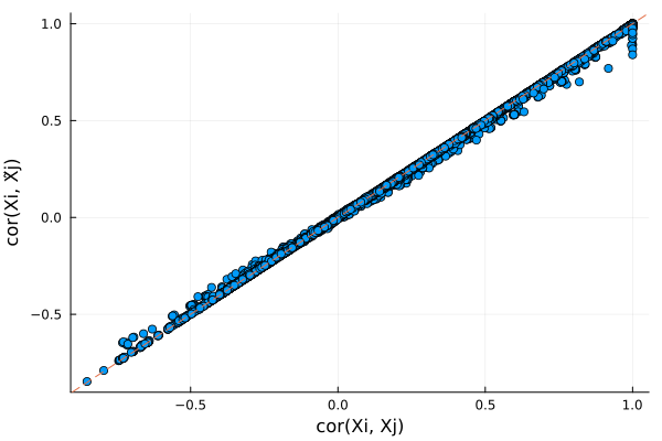

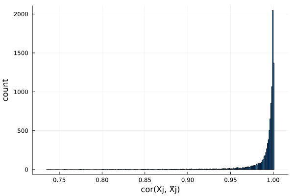
Plots distribution of $cor(X_j, \tilde{X}_j)$ for all $j$. Ideally, we want $cor(X_j, \tilde{X}_j)$ to be small in magnitude (i.e. $X$ and $\tilde{X}$ is very different). Here the knockoffs are tightly correlated with the original genotypes, so they will likely have low power.

r2 = Float64[]
for j in 1:size(X, 2)
    push!(r1, cor(@view(X[:, j]), @view(X[:, j])))
    push!(r2, cor(@view(X[:, j]), @view(X̃[:, j])))
end
histogram(r2, legend=false, xlabel="cor(Xj, X̃j)", ylabel="count")